Page 5 : Cores and Coils – Continued
| On this page we begin to discuss coil arrangements and magnetic properties. This will eventually lead us to rotor design; since how or what you want your motor to do will dictate the design of your rotor as well. In Fig 13 below we'll look at various coil locations, and discuss some observations. Lets go MYTHBUSTING ! |
|
|
|
|
|
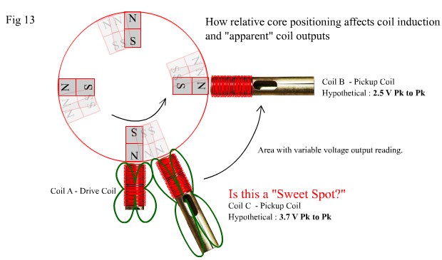
In Fig 13 above, there is a single drive coil and two pickup coils. With the motor turned on and spinning merrily we take measurements of the voltage in Coil B and Coil C. We notice that, although the coils are identical in every way, Coil C has a much higher Voltage than Coil B. Is this the "Sweet Spot" you dreamed about last night ? (LOL). As you move Coil C away from Coil A towards Coil B you notice the voltage drop until at the halfway mark you notice its nearly the same as Coil B. But as you get closer to Coil B, both Coil C and Coil B may increase their Voltage together. But they wont go as high as the Voltage was on Coil C , when it was near Coil A (the drive coil). Whats going on here ?? Simple induction, that's all: – represented by the green lines around Coils A and C. Theres no Punch without Judy! You cant stick one core near another, without shielding, and not have something happen between them when one or more is energised. Especially when the magnetic path between them is constantly changing due to a magnet swinging past at high speed. The magnet, as it passes from Coil A to Coil C is imparting some of the EMF and CEMF from Coil A on the leading and trailing edges of the pulse. Remember Coil A is turning on and off which is inducing a changing field exchange with Coil C . All the while this process of induction by proximity is happily facilitated by the closing of one end of the magnetic circuit between them by the magnet as it passes between them. So the higher Voltage reading is due to the Magnet and EMF/CEMF of Coil A combined. When Coil C is shifted right around to close proximity to Coil B, a field becomes shared between them which is induced by the magnet, and a similar sharing of Induced EMF occurs. Though not as profound, because neither coil is externally energised by a power supply like Coil A. But what comes in goes out. If you connect the ouputs of each coil to a load, then, when Coil C is near Coil A (the drive coil) it will deliver a higher power to the load. But the extra power will be drawn directly through induction from the drive Coil A, whilst Coil B will only deliver what it gets from the rotating magnet. When Coil C is near Coil B, they will both only deliver the same amount of energy as each other and the total energy combined will be less than the combination of Coil C and Coil A. This is because they are both now only receiving induced current from the magnet and not from Coil A. There is no "Sweet Spot" here without a sticky end. The higher power combination of Coil A and C together, fed into a load , results in higher current consumption from the driving source. In this case a battery supply. In Fig 14 below we look for another, different sort of "Sweet Spot ". See below Fig 14 for an explanation of this "Sweet Spot".
|
|
|
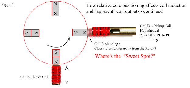
In Fig 14 above, we move the pickup Coil B towards and away from the moving rotor. All the while we are measuring the AC Voltage output of Coil B. Starting at about 1.5 centimetres away from the rotor, we notice we have a 1Volt peak to peak AC signal, and as we slowly push the core closer to the rotor we witness the voltage increase steadily until we are about 2-3 mm away from the rotor, and reach a Voltage of about 3.0 Volts. As we were moving the core closer to the rotor, we also noticed that the rotor slowed down just a "little bit". At 2-3 mm distance, we continue to push the coil closer to the rotor, and at first notice a slight increase in Voltage, but then all of a sudden the rotor begins to slow down significantly and the Voltage suddenly starts to drop off. As we slowly pull back on the coil and return it to the point where it was about 2-3 mm away, we notice the rotor regains its speed and the Voltage climbs back up to 3 Volts. Is this the "Sweet Spot" you dreamed about last night? (LOL). Well it might be, because it is a "Sweet Spot" in a sense. It is not a magical "OU" realm, but it is the right spot for your particular setup. The actual distance will depend on both the magnet strength and length and the nature of the core being used. But this particular "Sweet Spot" is present in all open magnetic systems. It does not affect Air Cored Coils until those coils are delivering current into a load. Even when that is the case, the effect is minimal on Air Cored Coils. To understand it we need to discuss the "Neutral Zone " and the "Transition Zone" which has not been discussed. Fig 15 below presents a diagramatic view of the Transition Zone
|
|
|
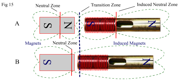
In Fig 15 above there are two groups of magnets to the left and cores to the right, which have become induced magnets. But there is a difference in the two groups A and B. In Fig 15 A the magnet and induced magnet are still acting as two individual magnets. The induced magnet's existence depends on the magnet, but it is a mirror image in every respect except absolute strength. As the magnet and core get closer, there is a movement in the Neutral Zones towards a common centre which is the Transition Zone. The neutral and transition zones only exist between two or more magnets or a magnet and a reactant core. They don't exist at all when a magnet is all alone and has no one to play with! "Or when two magnets become one!"
|
|
In Fig 15 B the core has moved so closely to the magnet, that it has breached the mutual transition Zone, and has now fallen entirely under the domain of the magnet's overwhelming influence. The two separate bodies, for all magnetic intents and purposes, have become "like one"! The induced Neutral Zone disappears as the entire core changes to a single magnetic polarity, and the Neutral Zone of the magnet plunges forward to assert it's new found dominant position. Prying the core and magnet apart now becomes harder work.. And they haven't even physically touched yet! This change is a quantum change that requires a leap in driving power to maintain rotor speed. The coercian factor involved in separating the two pieces is now affected by a change in magnetic state. When water changes to ice there is a quantum change in state to the individual water molecules. Think of the way that water has a "latent" heat quota, which must be extracted before it will turn to ice, (relate to creating electrical Coercian). Once it does turn to ice, that same latent heat quota must be filled (relate to creating Drag) before it will turn back into water again. All the while, you could have just left it alone, and you would have had a drink of water a whole lot quicker! Tuning in your pick-up coils to the "Right Spot" is strongly recommended. You will get the maximum Voltage and Current without paying a greater price than you need to. I also recommend, that you start off your construction by mounting your Drive Coils first. Play around with the Drive coils to "tune them in" to the "Right Spot", which is the best distance from the rotor. The best distance in this case, will be when you are getting the Maximum desirable RPM from a Minimum Current Draw for that given Maximum desirable RPM. Then, mount your pick-up coils and tune them in to the best distance that suits them. If the Drive Coils and Pick-Up Coils are identical, then the best distance will be the same for both coil types. Standard Electrical Induction Generator Theory says you should put the cores as close as possible. In this instance I strongly disagree. I say put them where you get the most Voltage before your rotor slows significantly. And remember – This is an Open Magnetic System and We Play by Different Rules here! What can appear to be a weakness can be a great strength. There is a "yet to be discussed anomoly" which makes good use of the changing Bloch and Transition Zones. Before moving on to working models using both Singular and Bi-Filar Coils, we will look at one more "Sweet Spot". Fig 16 below shows different results to be expected when the firing "pulse angle" changes due to shifts in the location of the Hall IC which is responsible for switching your pulses on and off at the correct time. |
|
|
|
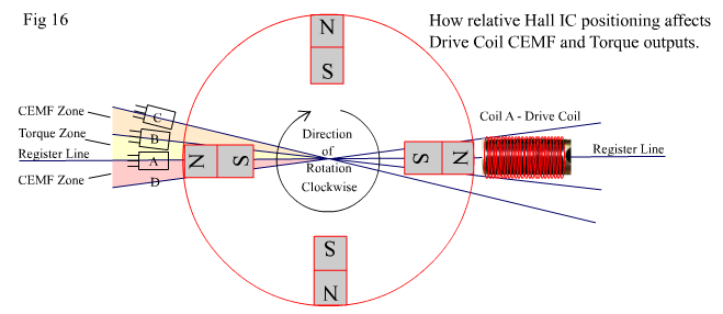
In Fig 16 above, there is a single drive coil mounted on one side of the rotor, and a Hall IC which provides the switching on the opposite side of the rotor. This alignment is for the ease of showing the different "Zones" created by changing the firing angle of the Hall IC. At point A the IC is in line with the "register point" of the magnet and coil. As you move away from the register point to point B, you will find that the RPM of the motor doesn't fall, or falls only very slightly, but the driving current also reduces slightly. When you go past point B and continue to approach point C you will notice the RPM will fall more rapidly, and driving current will begin to increase more rapidly. If you proceed past point C, RPM will fall dramatically and drive current consumption will increase dramatically. For maximum RPM and true Torque, the motor will run best if the Hall IC is just past the register point and no further than point B. Within that small angle range will be the optimum angle for your motor. The ACTUAL angle or angles are not predictable as a mandatory angle for all motors, but will vary according to other factors such as the width of your magnets with respect to the distance between them (duty cycle), and the strength of the magnets, the biasing of the Hall and so on. All you need to do, is measure your current consumption while you are varying the position, and you will find the angle which delivers the most RPM and torque for the minimum drive current. Between point B and C, there is a shift in the dynamics of the motor which translates torque availability to CEMF availability. Now there is always going to be a level of CEMF available while the coil is pulsing on and off. But the maximum level of usable CEMF (note* – current: not just potential) can be found when the motor is slightly "de-tuned" and your Hall IC is somewhere in the zone between B and C. But as mentioned, there will be a slight increase in current consumption, and a decrease in true torque. You will also notice point D. If the Hall IC was in this position before startup, then the rotor would turn anti-clockwise when the circuit was connected. But what happens in this area between point A and D, when you already have the motor spinning clockwise? For a small number of degrees past register in the opposite direction, a running motor can be quite forgiving and still run at high RPM. One thing to be noticed here, is that in this small region, the effect is the same as that between points B and C. By now, you should be starting to see that there's more to designing an "Adams" motor than first expected. Exactly what is it that you want from this motor? As I have previously mentioned, it is a very "Dynamic" motor, in every sense of the word, and what you design will be predicated by what you desire from it. But they are a great type of motor to experiment with due to the relative ease with which they can be made. A lot can be learned about motors in general by experimenting with them, and they also have the capability of introducing the beginner to simple semi-conductor electronic theory. |
|
|
|
Next…….To Bi or not to Bi ?
|